Introduction
In this final module, we learned to use random processes and L-systems to generate fractals. Those random processes involve applying functions to points iteratively, and they sometimes result in complex distinguished shapes like Barnsley Fern and Sierpinski's triangle. L-systems are composed of initial characters, the "axiom", and a set of rules that are applied to each character. By iteratively applying these rules, one can also create fractal patterns, like Hilbert's curve.
Results & Analysis
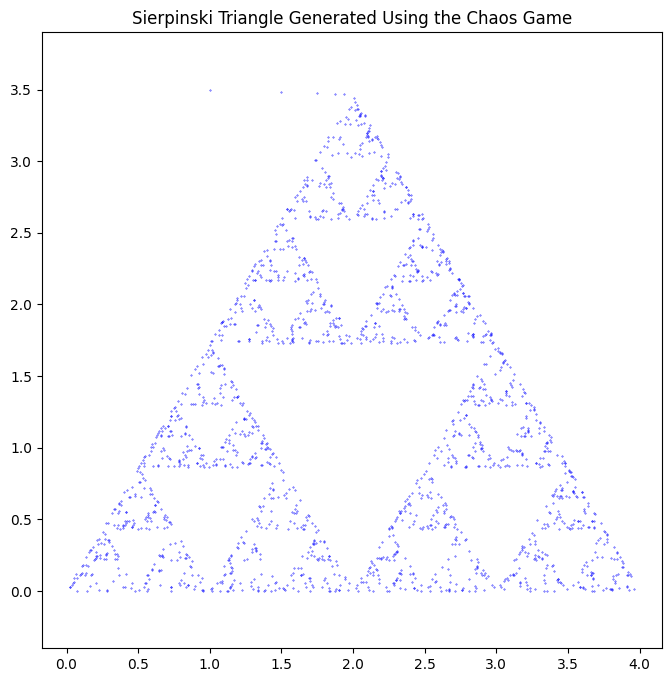
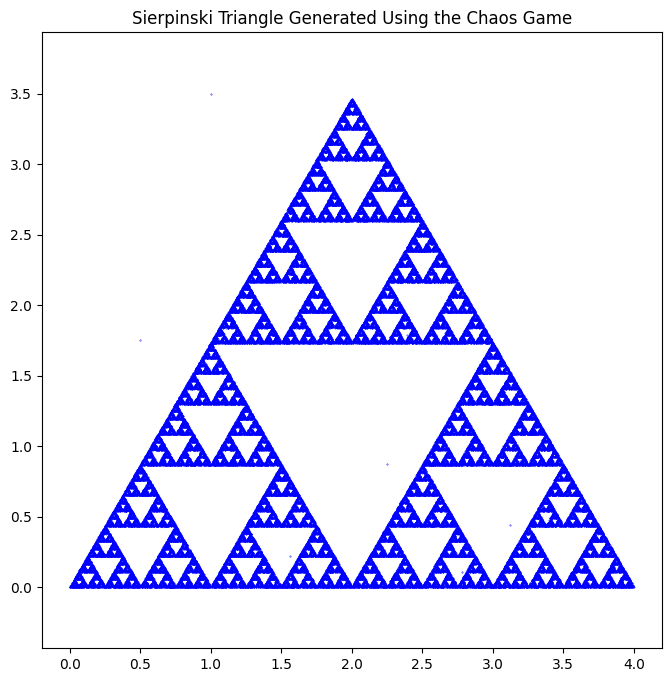
To generate the Sierpinski Triangle, we first set up the vertices, and a midpoint function to return the midpoint of two points. Now the iterative process is as follows: we pick a random starting point and then randomly select a vertex. Then we apply the midpoint function and the result is the next point in the list. We repeat this until we reach the desired number of iterations and we have the Sierpinski Triangle.
	import matplotlib.pyplot as plt
from random import random, randint #importing libraries
import numpy as np

def midpoint(P, Q):
    return (0.5*(P[0] + Q[0]), 0.5*(P[1] + Q[1]))

vertices = [(0, 0), (2, 2*np.sqrt(3)), (4, 0)]  #sets up vertices
iterates = 2000                                 #number of iterations
x, y = [0]*iterates, [0]*iterates               #lists with 0s of size iterates
x[0], y[0] = 1, 3.5                             #initial point

for i in range(1, iterates):

    k = randint(0, 2)

    x[i], y[i] = midpoint( vertices[k], (x[i-1], y[i-1]) )

plt.figure(figsize=(8, 8))
plt.scatter(x, y, color = 'b', s=0.1)
plt.title('Sierpinski Triangle Generated Using the Chaos Game')
plt.axis('equal')  # Ensure aspect ratio is equal for an equilateral triangle
plt.show()
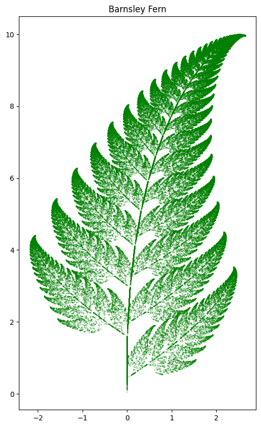
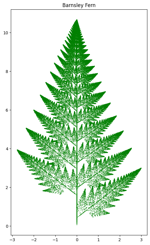
For Barnsley's Fern, we first define four functions that will move points differently and we associate probabilities to each function to determine what portion of the points will be moved by it. One function takes the points to the stem of the fern, one makes an order smaller fern and attaches it to the top of the stem, and the other two attach the two bottom leaves of the fern.
	import random
import matplotlib.pyplot as plt

# Define the transformation functions
def f1(x, y):     #stem
    x = 0
    y = 0.16 * y
    return x, y

def f2(x, y):           #smaller order copy
    x_new = 0.85 * x + 0.04 * y
    y_new = -0.04 * x + 0.85 * y + 1.6
    return x_new, y_new

def f3(x, y):         #left bottom leaf
    x_new = 0.2 * x - 0.26 * y
    y_new = 0.23 * x + 0.22 * y + 1.6
    return x_new, y_new

def f4(x, y):          #right bottom leaf
    x_new = -0.15 * x + 0.28 * y
    y_new = 0.26 * x + 0.24 * y + 0.44
    return x_new, y_new

# Probabilities for each function
probabilities = [0.01, 0.85, 0.07, 0.07]

# Barnsley Fern function
def barnsley_fern(iterations):
    x, y = 0, 0
    points = []

    for _ in range(iterations):
        rand = random.random()
          if rand   < sum(probabilities[:1]):    #pick f1 if rand lt 0.01
            x, y = f1(x, y)
        elif rand < sum(probabilities[:2]):    #pick f2 if rand 0.01 leq rand lt 0.86
            x, y = f2(x, y)
        elif rand < sum(probabilities[:3]):    #pick f3 if rand 0.86 leq rand lt 0.93
            x, y = f3(x, y)
        else:
            x, y = f4(x, y)                    #pick f4 if rand 0.93 leq rand lt 1

        points.append((x, y))                  #append list

    return points

# Generate points for the Barnsley Fern
iterations = 100000
fern_points = barnsley_fern(iterations)

# Plot the Barnsley Fern
x_vals, y_vals = zip(*fern_points)
plt.figure(figsize=(6, 10))
plt.scatter(x_vals, y_vals, s=0.1, color='green')
plt.title('Barnsley Fern')
plt.show()
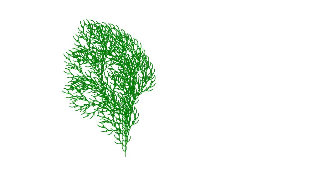
Next we learned how to use L-systems to create a tree being blown by wind. To accomplish this, first we set up a function to apply a set of rules to a character. Then we create another function that takes a single starting character, an "axiom," and outputs a string based on the rule set. This can be repeated iteratively to create fractal patterns.
	# Initialize the turtle
initializeTurtle()
showturtle()

# Function to apply L-system rules
def apply_rule(char, rules):                   #applies rule to character
    return rules.get(char, char)

# Function to generate L-system string
def generate_lsystem(axiom, rules, iterations):           #applies rule over a string
    current_string = axiom
    for _ in range(iterations):
        current_string = ''.join([apply_rule(char, rules) for char in current_string])
    return current_string

# Function to draw the L-system with turtle
def draw_lsystem(turtle_string, length, angle):      #defines what each character does
    stack = []
    for command in turtle_string:
        if command == 'F':                            #moves forward
            forward(length)
        elif command == '+':                          #turns left
            left(angle)
        elif command == '-':                          #turns right
            right(angle)
        elif command == '[':                          #saves the position like a checkpoint
            position = (getx(), gety())
            heading_angle = heading()
            stack.append((position, heading_angle))
        elif command == ']':                         #returns to the previously saved position
            position, heading_angle = stack.pop()
            jump(position[0], position[1])
            face(heading_angle)

# Define the L-system rules
rules = {'F': 'FF+[+F-F-F]-[-F+F+F]'}

axiom = 'F'
iterations = 4

# Generate the L-system string
turtle_string = generate_lsystem(axiom, rules, iterations)

# Set up the turtle
jump(400, 500)
face(0)
color('green')

# Draw the L-system fractal tree
length = 8
angle = 25
draw_lsystem(turtle_string, length, angle)

# Display the drawing
show()
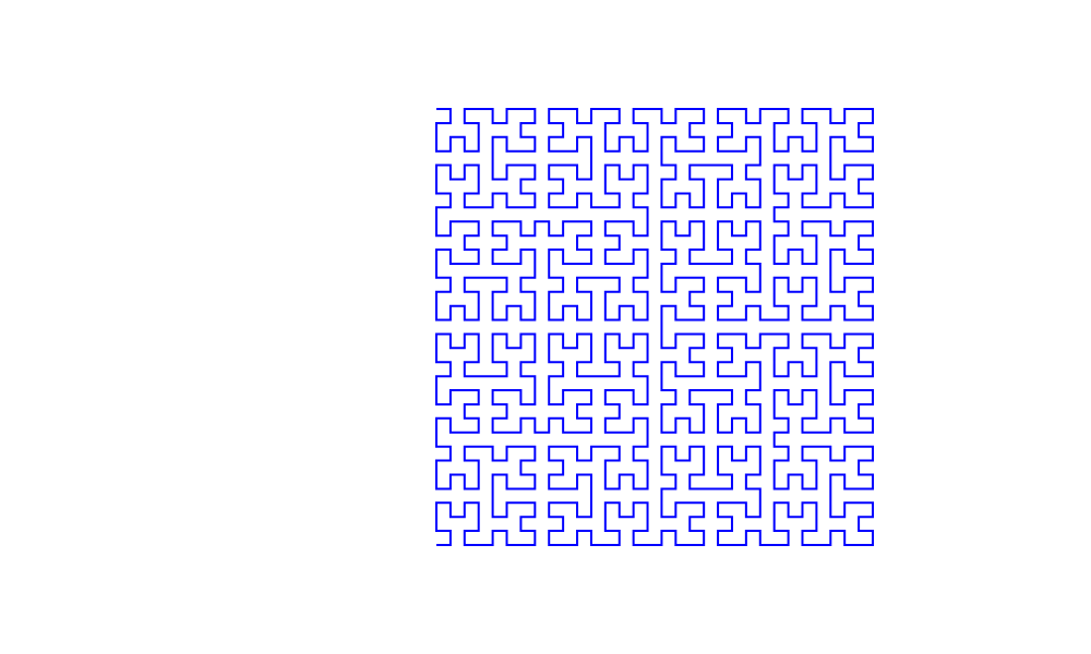
After getting familiar with L-systems, we turn to Hilbert curves. They are very special, since one can use them to fill a two dimensional square with a one dimensional continuous curve. That is why they are also called space-filling curves. The process is the same but with a different rule set.
	# Import necessary modules
import math

# Initialize the turtle
initializeTurtle()
showturtle()

# Function to apply L-system rules
def apply_rules(char, rules):
    return rules.get(char, char)

# Function to generate L-system string
def generate_lsystem(axiom, rules, iterations):
    current_string = axiom
    for _ in range(iterations):
        next_string = ''.join([apply_rules(char, rules) for char in current_string])
        current_string = next_string
    return current_string

# Function to draw the L-system with turtle
def draw_lsystem(turtle_string, length, angle):
    for command in turtle_string:
        if command == 'F':
            forward(length)
        elif command == '+':
            left(angle)
        elif command == '-':
            right(angle)
        # 'L' and 'R' are placeholders; we ignore them in drawing
        else:
            pass  # Ignore other characters

# Set the parameters for the Hilbert Curve
axiom = 'L'
rules = {
    'L': '-RF+LFL+FR-',
    'R': '+LF-RFR-FL+'
}
iterations = 5  # Adjust the iterations to change the order (e.g., 1 to 5)
angle = 90

# Generate the L-system string for the Hilbert curve
hilbert_string = generate_lsystem(axiom, rules, iterations)

# Calculate the step size based on desired size and iterations
size = 400  # Total size of the Hilbert curve (adjust as needed)
n = 2 ** iterations - 1
length = size / n

# Move to starting position
jump(400, 500)  # Adjust the starting position to fit your canvas
face(0)
color('blue')

# Draw the Hilbert curve
draw_lsystem(hilbert_string, length, angle)

# Display the drawing
show()
Conclusion
In this module we learned how to generate fractal patterns using the chaos game and L-systems. Throughout the course, we learned many different ways to code and visualize fractal patterns, and also developed some HTML and Python skills. With these tools available, we are now prepared to manipulate and toy with fractal patterns in real life, an essential skill for scientists.